# Single Vector
fruit <- "papaya"

fruit
[1] "papaya"Still under construction.
In the Chapter 3, we learned about different data types in R such as double, integer, character, and logical. Just as we organize physical items, and organize our personal space - our data needs special containers to organize and store different types of data. These containers are called data structures.
Each data structure in R has specific characteristics:
[] or$Before exploring the different data structures, we have three functions that can help us understand the data structure. length() tells us the number of elements we have in one dimensional data structures, dim() tells us the number of rows and columns in a multidimensional data structure. Lastly, we have str() which gives information about the number of rows and columns, and the underlying data types for the columns with preview.
We’ve actually worked with atomic vectors, and we have been working with them since the start of this book. An atomic vector is the simplest data structure in R (Grolemund 2014). Think of it as a one-dimensional data that can hold only one type of data. Honestly, the different data types are actually atomic vectors. The simplest for of atomic vectors is the scalar vector which contains only one element.
# Single Vector
fruit <- "papaya"
fruit[1] "papaya"We can make our vectors longer using c().
# Multivalue vector
fruits <- c("papaya", "orange", "apple", "pineapple", "grape",
            "strawberries", "avocado")

fruits
[1] "papaya" "orange" "apple" "pineapple" "grape"
[6] "strawberries" "avocado" Since both fruit and fruits have one dimension we can use length() to get their number of elements.
length(fruit) # shows the number of element(s) in fruit[1] 1length(fruits) # shows the number of element(s) in fruits[1] 7Atomic vectors can only hold one data type at a time. In the example below, we created a new object of double data type, then combine it with the fruits object which we created earlier. Checking the data type of the new object new_data, only a the character data type is returned.
set.seed(123)
diameter <- round(rnorm(10, mean = 23.5, sd = 0.6), 2)
typeof(diameter)[1] "double"new_data <- c(fruits, diameter)
new_data [1] "papaya" "orange" "apple" "pineapple" "grape"
[6] "strawberries" "avocado" "23.16" "23.36" "24.44"
[11] "23.54" "23.58" "24.53" "23.78" "22.74"
[16] "23.09" "23.23" typeof(new_data)[1] "character"Simple operations like addition, subtraction, multiplication, division, and so on, are the operations that can be performed on vectors. We can also use functions on them as shown in Chapter 4.
# Arithmetic Operation
x <- 15
y <- 20
y + x[1] 35y %% x[1] 5y / x[1] 1.333333Working with different data types that doesn’t mix well could be the only stumbling blocks in these simple operations.
"man" * 5Error in "man" * 5: non-numeric argument to binary operatorIn general character and numeric data types don’t mix, logical mixes with all data types.
To access a value in a vector we can get it with its index number. Indexing allows us access, slice, subset or modify specific elements in different data structures. We use the square brackets [] to specify the index position of elements we are interested in. The index position starts with 1, the index position of elements in fruits is show in Figure 5.1.
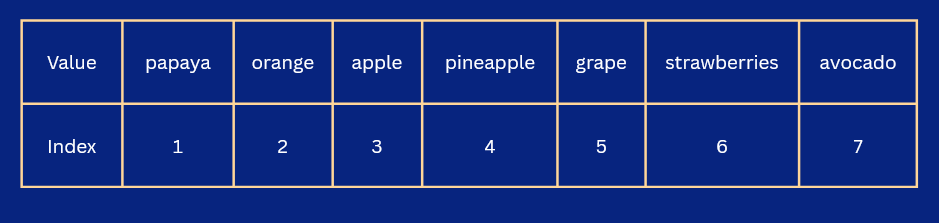
fruits vector
To get the first element papaya in the fruits vector, we specify its index position. As seen in Figure 5.1, the index of papaya is 1 in this case.
fruits[1][1] "papaya"To return multiple values at the same time, we combine those values with c() and pass it to the square brackets. To return avocado, grape, and orange, we select them by index position.
# select elements by specific position
fruits[c(7, 5, 2)][1] "avocado" "grape" "orange" We can also select a range of elements using :. To select elements from orange to grape, we do the following:
# select the range of elements that fall within that number.
fruits[2:5] [1] "orange" "apple" "pineapple" "grape" There are two ways to modify new elements in a vector:
append() function[]append() FunctionWe can use append() to add elements to a vector. The elements are usually added to the end of the vector. append() takes three arguments, x, the vector that you want to add a value(s) to, values, the new value(s) you want to add to the vector, and after, which determines the index position where you want the new value(s) slotted into.
append(x = fruits, values = "banana", after = 5) # adding new value in index position 5[1] "papaya" "orange" "apple" "pineapple" "grape"
[6] "banana" "strawberries" "avocado" Multiple values can be added when they are combined with c(). If the after argument is left empty, the new values are automatically placed at the end of the vector.
new_fruits <- c("kiwi", "grape", "cherry", "mango", "peach")
append(fruits, new_fruits) [1] "papaya" "orange" "apple" "pineapple" "grape"
[6] "strawberries" "avocado" "kiwi" "grape" "cherry"
[11] "mango" "peach" []To add a new value using the square bracket you have to assign the value to the index position you want the new value to occupy.
fruit[2] <- "mango" # add new element to a new index number
fruit[1] "papaya" "mango" If you insert an index that is more than the very next index number, you get the index positions filled with NA until the position you specified.
fruit[5] <- "Clementine"
fruit[1] "papaya" "mango" NA NA "Clementine"To prevent this, you can use a simple trick. Simply pass the length of the fruit + 1 into the square bracket when you want to add a new value to the last position.
fruit[length(fruit)+1] <- "Guava"
fruit[1] "papaya" "mango" NA NA "Clementine"
[6] "Guava" You can also remove elements of a vector using the square bracket. You do this by passing a negative value into the index number
fruit[-4] # Show values left after removing first value.[1] "papaya" "mango" NA "Clementine" "Guava" fruit <- fruit[-1] # Reassign to variable to confirm the change.
fruit[1] "mango" NA NA "Clementine" "Guava" The square brackets is also used to change the values of object using their index position.
fruit[3] # Position to be changed[1] NAfruit[3] <- "tomato" # Replace avocado with tomato
fruit # new elements[1] "mango" NA "tomato" "Clementine" "Guava" Multiple positions can also be changed by using c() or using : for a sequence of index position.
fruit[2:3] <- c("cayenne", "pomegranate")
fruit[1] "mango" "cayenne" "pomegranate" "Clementine" "Guava" Using [] offers more flexibility than append(), as it can be used to add, change and remove the elements of a vector.
There are instances where we perform operations such as converting from one unit to the other. In the case where our recorded values are more than one, which is usually the case, we would like to convert all of them with a single value. For example: An experiment is designed to evaluate the impact of various feed formulations on the weight gain and overall health of pigs, with the objective of selecting the optimal diet for a new litter to maximize growth and well-being. The weights of 40 pigs that have been administered feed_x for 3 months is given below.
set.seed(123)
feed_x <- round(rnorm(n = 40, mean = 87000, sd = 10000), 2)
feed_x [1] 81395.24 84698.23 102587.08 87705.08 88292.88 104150.65 91609.16
[8] 74349.39 80131.47 82543.38 99240.82 90598.14 91007.71 88106.83
[15] 81441.59 104869.13 91978.50 67333.83 94013.56 82272.09 76321.76
[22] 84820.25 76739.96 79711.09 80749.61 70133.07 95377.87 88533.73
[29] 75618.63 99538.15 91264.64 84049.29 95951.26 95781.33 95215.81
[36] 93886.40 92539.18 86380.88 83940.37 83195.29The value gotten was recorded in grams and we prefer the kilogram. To do this, we simply divide by a 1000
feed_x_kg <- round(feed_x / 1000, 2)
feed_x_kg [1] 81.40 84.70 102.59 87.71 88.29 104.15 91.61 74.35 80.13 82.54
[11] 99.24 90.60 91.01 88.11 81.44 104.87 91.98 67.33 94.01 82.27
[21] 76.32 84.82 76.74 79.71 80.75 70.13 95.38 88.53 75.62 99.54
[31] 91.26 84.05 95.95 95.78 95.22 93.89 92.54 86.38 83.94 83.20This is possible because the operation is carried out element-wise, and a phenomenon called vector recycling is happening. In vector recycling, vectors of shorter length are repeated multiple times to match up with longer vectors. As long as the longer vector is a multiple of the short vector, we get no warning message as we have below.
feed_x_kg * c(0.1, 0.5) [1] 8.140 42.350 10.259 43.855 8.829 52.075 9.161 37.175 8.013 41.270
[11] 9.924 45.300 9.101 44.055 8.144 52.435 9.198 33.665 9.401 41.135
[21] 7.632 42.410 7.674 39.855 8.075 35.065 9.538 44.265 7.562 49.770
[31] 9.126 42.025 9.595 47.890 9.522 46.945 9.254 43.190 8.394 41.600If the longer vector is not a multiple, we get a warning message and the result gets computed regardless, but there will be a cut off in operation.
feed_x_kg / c(0.3, 0.3, 0.4)Warning in feed_x_kg/c(0.3, 0.3, 0.4): longer object length is not a multiple
of shorter object length [1] 271.3333 282.3333 256.4750 292.3667 294.3000 260.3750 305.3667 247.8333
[9] 200.3250 275.1333 330.8000 226.5000 303.3667 293.7000 203.6000 349.5667
[17] 306.6000 168.3250 313.3667 274.2333 190.8000 282.7333 255.8000 199.2750
[25] 269.1667 233.7667 238.4500 295.1000 252.0667 248.8500 304.2000 280.1667
[33] 239.8750 319.2667 317.4000 234.7250 308.4667 287.9333 209.8500 277.3333While recycling can be useful, it can also leads to wrong results, so ensure you check if there are warnings and your results are as expected.
A matrix is a two-dimensional data structure that holds elements of the same data type arranged in rows and columns. Think of it as a calendar with with just numbers. To create a matrix, use the matrix() function. Since it is two dimensional, you have to specify the number of rows and columns you want. You can specify the number of rows with nrow and the number of columns with ncol.
mat <- matrix(1:6, nrow = 2, ncol = 3)
mat [,1] [,2] [,3]
[1,] 1 3 5
[2,] 2 4 6If you use only one of nrow or ncol, the other gets filled automatically. For example we can create a simple calendar month.
my_calendar <- matrix(1:30, ncol = 7)Warning in matrix(1:30, ncol = 7): data length [30] is not a sub-multiple or
multiple of the number of columns [7]my_calendar [,1] [,2] [,3] [,4] [,5] [,6] [,7]
[1,] 1 6 11 16 21 26 1
[2,] 2 7 12 17 22 27 2
[3,] 3 8 13 18 23 28 3
[4,] 4 9 14 19 24 29 4
[5,] 5 10 15 20 25 30 5The calendar looks weird and that’s because the numbers are usually filled by columns. To change this arrangement, set the byrow to TRUE
my_calendar <- matrix(1:30, ncol = 7, byrow = TRUE)Warning in matrix(1:30, ncol = 7, byrow = TRUE): data length [30] is not a
sub-multiple or multiple of the number of columns [7]my_calendar [,1] [,2] [,3] [,4] [,5] [,6] [,7]
[1,] 1 2 3 4 5 6 7
[2,] 8 9 10 11 12 13 14
[3,] 15 16 17 18 19 20 21
[4,] 22 23 24 25 26 27 28
[5,] 29 30 1 2 3 4 5Now this looks more like a calendar. But an incomplete calendar, we need the names of the day, and also the week numbers. We will get to this in the next section, but let’s address something else which you will come across a lot. That is creating matrix from vector objects. We make a matrix from a vector by passing it to the matrix() function and giving a value to either of nrow or ncol.
fruit_mat <- matrix(fruits, nrow = 4) # make matrix from fruits vectorWarning in matrix(fruits, nrow = 4): data length [7] is not a sub-multiple or
multiple of the number of rows [4]fruit_mat [,1] [,2]
[1,] "papaya" "grape"
[2,] "orange" "strawberries"
[3,] "apple" "avocado"
[4,] "pineapple" "papaya" To get the dimension of matrix use dim() function.
dim(fruit_mat)[1] 4 2The result [1] 4 2 is interpreted 4 by 2, i.e. four rows and two column. That matrix is thereby called a 4 by 2. The object my_calendar is having 5 rows by 7 columns, that makes it a 5 by 7 matrix
A property of matrix is being two dimensional. From the current result of the calendar, we have [1,] and [,1] signifying rows and columns respectively. These numbers are the column and row indices of a matrix and they can replaced with names of our choosing using the colnames() and rownames() functions.
colnames(my_calendar) <- c("Mon", "Tues", "Wed", "Thurs", "Fri", "Sat", "Sun")
rownames(my_calendar) <- paste("Week", 1:5)
my_calendar Mon Tues Wed Thurs Fri Sat Sun
Week 1 1 2 3 4 5 6 7
Week 2 8 9 10 11 12 13 14
Week 3 15 16 17 18 19 20 21
Week 4 22 23 24 25 26 27 28
Week 5 29 30 1 2 3 4 5Now my_calendar looks more like a calendar.
Similar to vectors, matrix can perform arithmetic operations. For arithmetic with scalar vector, the operation is carried on each element of the matrix.
my_mat <- matrix(1:6, nrow = 3)
my_mat [,1] [,2]
[1,] 1 4
[2,] 2 5
[3,] 3 6my_mat * 5 [,1] [,2]
[1,] 5 20
[2,] 10 25
[3,] 15 30my_mat - 15 [,1] [,2]
[1,] -14 -11
[2,] -13 -10
[3,] -12 -9my_mat2 <- matrix(2:7, nrow = 3)
my_mat2 / my_mat [,1] [,2]
[1,] 2.000000 1.250000
[2,] 1.500000 1.200000
[3,] 1.333333 1.166667Matrix with unequal dimension cannot be added together
my_mat3 <- matrix(7:15, nrow = 3)
my_mat3 [,1] [,2] [,3]
[1,] 7 10 13
[2,] 8 11 14
[3,] 9 12 15my_mat3 + my_matError in my_mat3 + my_mat: non-conformable arraysLike with vectors, you can access any particular element in a matrix using the square brackets, []. Since matrix is two dimensional, there’s a little adjustment in how we access elements as we have to specify rows and columns. The syntax is [row_index, column_index]. For example, let’s access the third row and second column element of fruit_mat.
fruit_mat [,1] [,2]
[1,] "papaya" "grape"
[2,] "orange" "strawberries"
[3,] "apple" "avocado"
[4,] "pineapple" "papaya" fruit_mat[3, 2][1] "avocado"We can also access more than one element of a particular axis (row and column) by passing in a vector.
fruit_mat[c(1, 3, 2), 1] # This returns row 1, 3, and 2 elements of column 1[1] "papaya" "apple" "orange"fruit_mat[2, c(1, 2)][1] "orange" "strawberries"You can also use : within an axis to access elements within a range
fruit_mat[2:4, c(1, 2)] # returns row 2, 3, and 4 element of column 1 and 2. [,1] [,2]
[1,] "orange" "strawberries"
[2,] "apple" "avocado"
[3,] "pineapple" "papaya" To return all the rows of a particular column, leave the row space within the square bracket empty, and specify the index of the column you want to return
fruit_mat[,1][1] "papaya" "orange" "apple" "pineapple"fruit_mat[,2][1] "grape" "strawberries" "avocado" "papaya" To return all the columns of a particular row, the column space is left empty.
fruit_mat[3:4, ] # returns element of row 3 and 4 for all the columns. [,1] [,2]
[1,] "apple" "avocado"
[2,] "pineapple" "papaya" You can also access an element using the row and column names.
my_calendar["Week 2", ] Mon Tues Wed Thurs Fri Sat Sun
8 9 10 11 12 13 14 To add new columns to a matrix use cbind() and to add rows use rbind(). We’ll create a new matrix of fruits to show this .
new_fruit_list <- matrix(c("raspberry", "blue berries",
"kiwi", "clementine"),
nrow = 4)
new_fruit_list [,1]
[1,] "raspberry"
[2,] "blue berries"
[3,] "kiwi"
[4,] "clementine" fruit_list <- cbind(fruit_mat, new_fruit_list)
fruit_list [,1] [,2] [,3]
[1,] "papaya" "grape" "raspberry"
[2,] "orange" "strawberries" "blue berries"
[3,] "apple" "avocado" "kiwi"
[4,] "pineapple" "papaya" "clementine" To prevent error when combining column-wise ensure the number of rows of the matrices to be joined are equal and the number of columns are equal when combining row-wise.
rbind(fruit_list, c("avocado", "pear", "lemon")) [,1] [,2] [,3]
[1,] "papaya" "grape" "raspberry"
[2,] "orange" "strawberries" "blue berries"
[3,] "apple" "avocado" "kiwi"
[4,] "pineapple" "papaya" "clementine"
[5,] "avocado" "pear" "lemon" Transposing matrix is done using t(). This flips row elements to columns and column elements to rows.
fruit_mat_transposed <- t(fruit_mat)
fruit_mat_transposed [,1] [,2] [,3] [,4]
[1,] "papaya" "orange" "apple" "pineapple"
[2,] "grape" "strawberries" "avocado" "papaya" dim(fruit_mat_transposed)[1] 2 4Data frames are two-dimensional like matrix and are one of the most common way to store data. They are similar to Excel spreadsheets in how they look. What makes data frames different from matrix is their ability to store different data types. To create a data frame, we use the data.frame() function.
data.frame(
x = 1:10,
y = letters[1:10],
z = month.abb[1:10]
) x y z
1 1 a Jan
2 2 b Feb
3 3 c Mar
4 4 d Apr
5 5 e May
6 6 f Jun
7 7 g Jul
8 8 h Aug
9 9 i Sep
10 10 j OctData frames can combine vectors into a table where each vector becomes a column. The vectors to be used have to be of the same length to avoid error.
fruit <- c("orange", "mango", "apple")
stock <- c(5, 3, 0)
available <- c(TRUE, TRUE, FALSE)
fruit_tbl <- data.frame(fruit, stock, available)
fruit_tbl fruit stock available
1 orange 5 TRUE
2 mango 3 TRUE
3 apple 0 FALSEElements in data.frame are accessed in a similar fashion as matrix with an extra tweak of their columns being accessible using the dollar sign $. Using the dollar sign returns the columns as a vector.
fruit_tbl$stock[1] 5 3 0When accessing a column with its name and the square bracket, it’s not necessary to include the comma when the name is in quotation marks. The column with the specified name will be returned. This is also the same when you use index number, once a comma is not included, the column is automatically returned
fruit_tbl["stock"]
fruit_tbl[2] stock
1 5
2 3
3 0 stock
1 5
2 3
3 0You can still use the commas to return specific rows and columns if you choose to, or return a particular observation as shown below:
fruit_tbl[2, 3][1] TRUEUsing the square brackets, and index number of the column we want to remove, we can remove old columns or add new columns to a data frame.
# Removing a Column
fruit_tbl[-1] stock available
1 5 TRUE
2 3 TRUE
3 0 FALSE# Adding a column
fruit_tbl["location"] <- c("online", "on site", "online")
fruit_tbl fruit stock available location
1 orange 5 TRUE online
2 mango 3 TRUE on site
3 apple 0 FALSE onlineA list is a versatile data structure that can store elements of different types and sizes - including other data structures like vectors, matrices, and even other lists. Think of it like a container that can hold different kinds of boxes.
# Basic list creation
my_list <- list(
fruits,
fruit_mat,
c(TRUE, FALSE),
FALSE,
fruit_mat_transposed,
fruit_tbl,
my_calendar
)
my_list[[1]]
[1] "papaya"       "orange"       "apple"        "pineapple"    "grape"
[6] "strawberries" "avocado"
[[2]]
     [,1]        [,2]
[1,] "papaya"    "grape"
[2,] "orange"    "strawberries"
[3,] "apple"     "avocado"
[4,] "pineapple" "papaya"
[[3]]
[1] TRUE FALSE
[[4]]
[1] FALSE
[[5]]
[,1] [,2] [,3] [,4]
[1,] "papaya" "orange" "apple" "pineapple"
[2,] "grape" "strawberries" "avocado" "papaya"
[[6]]
fruit stock available location
1 orange 5 TRUE online
2 mango 3 TRUE on site
3 apple 0 FALSE online
[[7]]
       Mon Tues Wed Thurs Fri Sat Sun
Week 1   1    2   3     4   5   6   7
Week 2   8    9  10    11  12  13  14
Week 3  15   16  17    18  19  20  21
Week 4  22   23  24    25  26  27  28
Week 5 29 30 1 2 3 4 5The objects in a list can be given a name using names() function.
names(my_list) <- c("fruits", "fruit_mat", "logical_1", "logical_2",
"fruit_transposed_matrix", "fruit_dataframe", "my_calendar_matrix")On printing list now, we’ll see each object named.
my_list$fruits
[1] "papaya" "orange" "apple" "pineapple" "grape"
[6] "strawberries" "avocado"
$fruit_mat
     [,1]        [,2]
[1,] "papaya"    "grape"
[2,] "orange"    "strawberries"
[3,] "apple"     "avocado"
[4,] "pineapple" "papaya"
$logical_1
[1] TRUE FALSE
$logical_2
[1] FALSE
$fruit_transposed_matrix
     [,1]     [,2]           [,3]      [,4]
[1,] "papaya" "orange"       "apple"   "pineapple"
[2,] "grape"  "strawberries" "avocado" "papaya"
$fruit_dataframe
   fruit stock available location
1 orange     5      TRUE   online
2  mango     3      TRUE  on site
3  apple     0     FALSE   online
$my_calendar_matrix
Mon Tues Wed Thurs Fri Sat Sun
Week 1 1 2 3 4 5 6 7
Week 2 8 9 10 11 12 13 14
Week 3 15 16 17 18 19 20 21
Week 4 22 23 24 25 26 27 28
Week 5 29 30 1 2 3 4 5The square bracket, [] is used to select elements in a list but to print the items in the object you use [[]]. Like data.frame you can also use the dollar sign, $,
my_list[1]$fruits
[1] "papaya"       "orange"       "apple"        "pineapple"    "grape"
[6] "strawberries" "avocado" Notice the difference when we use [[]]. The result is similar to using $ to access the objects within the list
my_list[[1]][1] "papaya" "orange" "apple" "pineapple" "grape"
[6] "strawberries" "avocado" my_list$fruits # similar to [1][1] "papaya" "orange" "apple" "pineapple" "grape"
[6] "strawberries" "avocado" To access the item in each object add a square bracket in front.
my_list[[1]][3][1] "apple"To confirm an object data structure, use their is.*() variant. For vectors, is.vector(), for matrix, is.matrix() and so on. To convert from one structure to another, use their as.*() variant. For vector as.vector(), for matrix, as.matrix() and so on.
is.vector(my_calendar)[1] FALSEis.vector(fruits)[1] TRUEis.matrix(my_calendar)[1] TRUEas.data.frame(my_calendar) Mon Tues Wed Thurs Fri Sat Sun
Week 1 1 2 3 4 5 6 7
Week 2 8 9 10 11 12 13 14
Week 3 15 16 17 18 19 20 21
Week 4 22 23 24 25 26 27 28
Week 5 29 30 1 2 3 4 5In this chapter you learned about data structures in R. You saw how to create each data structure, how to access the elements of each structure. Also, you learned how to add and remove items from each data structure. You got introduced to checking the properties of each data structure such as their length and dimensions. Next you will learn about packages in R and how to install them, after you will bring together the knowledge you’ve gathered from chapter one into making R Scripts and R projects.