"tree"[1] "tree"Now that we are familiar with the basic syntax of R and its syntax. We move on to different data types, and that’s because these operators works on one or more of these data types. Understanding the concept of the data types, reduces the likelihood of an error occurring, or in some case ease the debugging process when an error does occur. This is because one of the most common source of error when using R, or performing analysis in general regardless of the software used is wrong, inappropriate or inconsistent data types, read this blog post for more details.
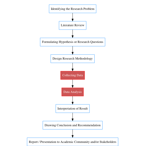
Researchers regardless of the field are analysts working with various forms of data, which can be survey responses, secondary data from institutions, and field or lab measurements among others. These data are usually any of numbers, response in form of alphabets, ranking, rating or choice response such as yes/no. It is crucial to understand the types of data you are working with before any analysis is done. In the research process Figure 3.1, data collection and analysis are key stages, and one that frustrates a lot of researcher. While data collection is often tedious, this should not be the same with data analysis. With a proper framework and workflow, analyzing your data should be less daunting than collecting it.
There are six different data types in R, five which we will come across frequently in this book. In R, the function typeof() and class() are used to check the data type of a variable, these functions will be useful as we move along. The data types are in R are:
Characters represent strings/texts and are written in R by enclosing contents in quotation marks. The quotation mark can either be the single ' or double " and anything can be a character as long its contents are wrapped in quotation mark.
"tree"[1] "tree"I’d advise to use the double " over the single ' as it allows you to use the apostrophe without worry, and it just also looks better.
'My boss said - "what makes a good boss is not knowing all, that's why I have employees"'Error in parse(text = input): <text>:1:66: unexpected symbol
1: 'My boss said - "what makes a good boss is not knowing all, that's
^The above code is wrong because of the apostrophe as it is mistaken as closing the character statement.
"My boss said - 'what makes a good boss is not knowing all, that's why I have employees'"[1] "My boss said - 'what makes a good boss is not knowing all, that's why I have employees'""The man's children" # Definitely looks better[1] "The man's children"'The man"s children'[1] "The man\"s children"We can check the data type of an object with either class() or typeof().
typeof("tree")[1] "character"class("tree")[1] "character"class("2")[1] "character"class("+")[1] "character"When we assign characters to a variable, the content of the variable will be evaluated and not the variable in its self. As explained in Chapter 2.4 variables are references and not a value in themselves.
tree <- "Quercus robur"
class(tree)
[1] "character"Let’s look at the example below, we have error because oak is an object with no values assigned to it. So oak and "oak" are different. The latter is a character while the former is an object.
class(oak)Error: object 'oak' not foundThere is a way to check if an objects is a character or not different from using class() and typeof(). The is.character() function returns a TRUE or FALSE used. TRUE, its a character data type and vice-versa.
is.character("moabi")[1] TRUEis.character(2)[1] FALSEis.character("2")[1] TRUEFactors are used to represent categorical data in R. They are usually leveled, and can only contain predefined values. The levels are usually distinct values. Data that can be represented as factors relates to responses like educational status, income level/class, satisfaction rating and so on. For example, in a farm of 5000 livestock, 2000 are goats, 390 cattles, 1500 sheeps, and 1100 pigs. The levels, i.e., the distinct animals in the farm include goat, sheep, pig, and cattle.
There are two types of factors or categorical data. We have ordered (ordinal) categorical data or unordered (nominal) categorical data. The function factor() is used to create factors in R.
These are unordered categorical data with levels. There’s no degree of distance or ranking in nominal factor variables. Example are the name of states in a country, name of trees, names of treatments, and so on. Below are example nominal data.
Treatment is a technical term used in research, if the word treatment seem unfamiliar to you at the moment, we will discuss it in the next part of this book.
livestock <- factor(c("pig", "cattle", "goat", "sheep", "sheep",
                       "sheep", "pig", "sheep","sheep",
                       "sheep", "pig", "pig", "goat", "goat", "cattle")
                     )
tree_names <- factor(c("Lophira alata", "Triplochiton scleroxylon",
                       "Mansonia altissima", "Celtis africana",
                       "Borassus aethiopum")
                     )
poultry_birds <-factor(c("breeders", "broilers", "layers"))
fertilizer <- factor(c("N", "P", "K"))
livestock [1] pig cattle goat sheep sheep sheep pig sheep sheep sheep
[11] pig pig goat goat cattle
Levels: cattle goat pig sheeptree_names[1] Lophira alata Triplochiton scleroxylon Mansonia altissima
[4] Celtis africana Borassus aethiopum
5 Levels: Borassus aethiopum Celtis africana ... Triplochiton scleroxylonpoultry_birds[1] breeders broilers layers
Levels: breeders broilers layersfertilizer[1] N P K
Levels: K N PThe function, c(), is used to combine values. More about c() will be discussed in Chapter 4
When we print this variables, notice the output, especially that of livestock, we see that Levels is included as part of the result with the categories arranged in alphabetical order. At a closer look, you see that livestock Levels returns only the distinct animals even while they appear more than once in the data.
Using the function levels() we can get this distinct values of a factor returned as character.
levels(tree_names)[1] "Borassus aethiopum" "Celtis africana"
[3] "Lophira alata" "Mansonia altissima"
[5] "Triplochiton scleroxylon"Using class() we can confirm the data type of these objects.
class(poultry_birds)[1] "factor"If we use the typeof() function instead we get integer,soon to be discussed in 3.3.1. This is because class() checks the object class, while typeof() storage mode or internal type of objects and the factors are built on top of integers.
typeof(tree_names)[1] "integer"Ordinal factors are different from nominal factors, as they indicate a degree of difference, hierarchy, rank or order. Before we proceed to creating ordinal factors, let’s get more understanding into the levels attribute of factors. When we created the nominal factors, we did not include the level argument, as R automatically does that for us. If we specify the level argument we take more control of how factors are organized dictating a particular print order. For example, let’s check the difference in how the levels are arranged in the gender object below:
gender_1 <- factor(c("m", "f"), levels = c("f", "m"))
gender_2 <- factor(c("m", "f"), levels = c("m", "f"))gender_1[1] m f
Levels: f mgender_2[1] m f
Levels: m fThe levels of gender_1 and gender_2 follows the arrangement specified in their levels argument. The output of gender_1 is also similar to running the code without the levels argument specified, i.e., arranged in alphabetical order. This knowledge will be important when we want to create ordinal factors. There are two ways to create ordinal factors. The first is using the ordered() function, and the second is passing TRUE to the ordered argument in factor. Let’s take a quick example of a response that include educational level. The survey question would be typically asked such that only one response is ticked - ” What’s your highest educational level attained.” The responses when recorded could be encoded using numbers such 1, 2, 3, and so on, or alphabets such as A, B, C, etc., to represent the levels. For this example, the 2011 International Standard Classification of education which categorize education level into 9 distinct classes will be useful (ISCED 2012) .
education_level <- factor(
  c(7, 8, 4, 2, 3, 3, 4, 1, 5, 4, 4, 7, 2, 6, 5,
    1, 2, 7, 7, 6, 0, 3, 3, 7, 8, 1, 0, 5, 3, 7, 7,
    0, 5, 8, 0, 5, 6, 2, 2, 0, 2, 2, 6, 1, 5, 0, 3,
    8, 8, 5),
  levels = c(0:8),
  ordered = TRUE
)

education_level
[1] 7 8 4 2 3 3 4 1 5 4 4 7 2 6 5 1 2 7 7 6 0 3 3 7 8 1 0 5 3 7 7 0 5 8 0 5 6 2
[39] 2 0 2 2 6 1 5 0 3 8 8 5
Levels: 0 < 1 < 2 < 3 < 4 < 5 < 6 < 7 < 8The data might not make sense to some people, and it should not. With a good data documentation, understanding what the data means becomes easier. Some could argue that it would be better to write the label outright without the stress of encoding them with numbers, and that’s a solid argument, but such data entry task could be daunting depending on the size of the project. There’s an easy way to go about this would be that makes the stress of retyping reduce with the labels argument. The labels argument replaces the numbers with texts/labels so they are easy to understand.
education_level_labelled <- factor(
  c(7, 8, 4, 2, 3, 3, 4, 1, 5, 4, 4, 7, 2, 6, 5,
    1, 2, 7, 7, 6, 0, 3, 3, 7, 8, 1, 0, 5, 3, 7, 7,
    0, 5, 8, 0, 5, 6, 2, 2, 0, 2, 2, 6, 1, 5, 0, 3,
    8, 8, 5),
  levels = c(0:8),
  labels = c("Early childhood", "Primary", "Lower secondary",
             "Upper secondary", "Post secondary non-tertiary",
             "Short cycle tertiary", "Bachelors", "Masters",
             "Doctoral"),
  ordered = TRUE
)

education_level_labelled
[1] Masters Doctoral
[3] Post secondary non-tertiary Lower secondary
[5] Upper secondary Upper secondary
[7] Post secondary non-tertiary Primary
[9] Short cycle tertiary Post secondary non-tertiary
[11] Post secondary non-tertiary Masters
[13] Lower secondary Bachelors
[15] Short cycle tertiary Primary
[17] Lower secondary Masters
[19] Masters Bachelors
[21] Early childhood Upper secondary
[23] Upper secondary Masters
[25] Doctoral Primary
[27] Early childhood Short cycle tertiary
[29] Upper secondary Masters
[31] Masters Early childhood
[33] Short cycle tertiary Doctoral
[35] Early childhood Short cycle tertiary
[37] Bachelors Lower secondary
[39] Lower secondary Early childhood
[41] Lower secondary Lower secondary
[43] Bachelors Primary
[45] Short cycle tertiary Early childhood
[47] Upper secondary Doctoral
[49] Doctoral Short cycle tertiary
9 Levels: Early childhood < Primary < Lower secondary < ... < DoctoralNow, this is easier to understand.
Let’s switch our attention back to ordinal factors. First, we set the ordered argument within factor to TRUE and a closer look at the Levels shows a different output. We have the lesser than symbol, which shows that Early childhood is lesser than Primary, Primary lesser than Lower secondary and so on. This represents a rank. Here, Early childhood is the lowest rank and Doctoral the highest rank. Using the function table() we can take a frequency of the response.
table(education_level_labelled)education_level_labelled
Early childhood Primary
6 4
Lower secondary Upper secondary
7 6
Post secondary non-tertiary Short cycle tertiary
4 7
Bachelors Masters
4 7
Doctoral
5 Specifying the levels is important as it also helps us detect if a level is missing.
edu_level <- factor(
  c(1, 2, 3, 4, 1, 1, 2, 3, 7, 8),
  levels = c(0:8),
  labels = c("Early childhood", "Primary", "Lower secondary",
             "Upper secondary", "Post secondary non-tertiary",
             "Short cycle tertiary", "Bachelors", "Masters",
             "Doctoral"),
  ordered = TRUE
)

edu_level
[1] Primary Lower secondary
[3] Upper secondary Post secondary non-tertiary
[5] Primary Primary
[7] Lower secondary Upper secondary
[9] Masters Doctoral
9 Levels: Early childhood < Primary < Lower secondary < ... < DoctoralEven when missing some levels, the Levels are still shown. In the current version of education level, edu_level, Early childhood, Bachelors, and Short cycle tertiary education levels are missing. Using table() shows this better.
table(edu_level)edu_level
Early childhood Primary
0 3
Lower secondary Upper secondary
2 2
Post secondary non-tertiary Short cycle tertiary
1 0
Bachelors Masters
0 1
Doctoral
1 We have been using functions like c(), table(), class() and so on for a while now without properly introducing functions properly. Just keep in mind that functions are variables with parenthesis in front of them. They are block of codes that perform specified actions. More will be discussion on that in Chapter 4.
To confirm if a variable is a factor data type use the is.factor() . Let’s create a new survey response, but this time it won’t be wrapped in the factor variable.
edu_level_chr <- c("Early childhood", "Primary", "Lower secondary",
                            "Upper secondary", "Post secondary non-tertiary",
                            "Short cycle tertiary", "Bachelors", "Masters",
"Doctoral")is.factor(edu_level_chr)[1] FALSEis.factor(livestock)[1] TRUEWe can also confirm if a factor is ordered or not using the function is.ordered()
is.ordered(edu_level)[1] TRUEIt is important to take a closer look at the output of your codes it shows if the output is what you expect. Factors have no quotation marks when returned, but characters do. This is a good distinction to keep in mind.
Numeric data are digits. There are two types of numeric data; integer and double.
Integer are whole numbers and are written by writing a digit followed by a L.
5L[1] 5class(5L)[1] "integer"When divided by another integer or another numeric data type the result is usually a double.
25L/5L[1] 5typeof(25L / 5L)[1] "double"Just like characters and factors, we can also check if a particular object is an integer using is.integer().
is.integer(5)[1] FALSEis.integer(5L)[1] TRUEDoubles are also referred to as floats. They are numbers with decimal point.
5.1[1] 5.1typeof(5.1)[1] "double"When a mathematical operation is performed on a double, a double is return
typeof(1.5/3)[1] "double"To check if an object is a double we use its is._ variant, in this case is.double()
is.double(2.9)[1] TRUEA sequence of integers or doubles can be created using : with the start on the left and the end at the right of the symbol.
1:15 [1] 1 2 3 4 5 6 7 8 9 10 11 12 13 14 15As is.integer() returns true for all integers and is.doubl()e returns true for doubles, is.numeric() returns true for all both types of data.
is.numeric(5L)[1] TRUEis.numeric(3.5)[1] TRUELogical data type are also referred to as Boolean values. Logical includes TRUE, FALSE and NA which means Not Available.
class(TRUE)[1] "logical"class(NA)[1] "logical"class(FALSE)[1] "logical"In Chapter 2.2, we saw that comparison operators always returns a logical operator as their result. We can also check the type as it is evaluated.
class(5 > 2)[1] "logical"5 > 2 is first evaluated which returns TRUE, then the class() of the result is checked which returns TRUE. In R, the deepest of the nested expressions are evaluated first and evaluated outwardly to the umbrella expression. We can also check for a logical value using is.logical()
is.logical(20 < 3)[1] TRUEis.logical(NA)[1] TRUEWe will not use the complex data type and its unlikely to analyze these type of data. Complex data types are numbers with an imaginary term i added to them
5i[1] 0+5i1 + 5i[1] 1+5itypeof(3i)[1] "complex"typeof(5 + 2i)[1] "complex"Similar to other data types, we can confirm if a data is a complex by using is.complex()
is.complex(5i)[1] TRUEIn R we can change data types using as.data_type similar to is.* which is used to check a data type.
tree_height <- 20:40
tree_height
[1] 20 21 22 23 24 25 26 27 28 29 30 31 32 33 34 35 36 37 38 39 40typeof(tree_height)[1] "integer"The above can be changed to a double using as.double() and back to integer using as.integer()
tree_height_2 <- as.double(tree_height)
typeof(tree_height_2)
[1] "double"We can also change characters to factors and factors to characters in a similar way
tree_names <- c("terminalia", "eucalyptus", "iroko", "oak")
class(tree_names)
[1] "character"To change the above to factor data type we’ll use the as.factor() function.
tree_names_fct <- as.factor(tree_names)

class(tree_names_fct)
[1] "factor"We can change this back to character by using as.character().
tree_names_chr <- as.character(tree_names_fct)
class(tree_names_chr)
[1] "character"as.character() can be used to coerce any data type to a character
tree_height [1] 20 21 22 23 24 25 26 27 28 29 30 31 32 33 34 35 36 37 38 39 40class(tree_height)[1] "integer"tree_height_chr <- as.character(tree_height)
class(tree_height_chr)[1] "character"Characters can be changed back to numeric or double data type using the as.double(), as.integer() or as.numeric() function. The functions will return a number only if what is been converted contains only digits, else, NA is returned as the result. we get a warning when there’s not a digit in the object being converted.
tree_height <- c(10, 15, 20, "25m")
tree_height
[1] "10" "15" "20" "25m"class(tree_height)[1] "character"tree_height <- as.double(tree_height)Warning: NAs introduced by coerciontree_height[1] 10 15 20 NAclass(tree_height)[1] "numeric"we can also convert factors to integers. As said in 3.2, factors are built on integers.
fruits <- factor(c("clementine", "kiwi", "avocado"))
class(fruits)
[1] "factor"as.integer(fruits)[1] 2 3 1We can also convert other data types to logical data type. All other numbers evaluate to TRUE either if they are positive or negative except zero which evaluates to zero.
as.logical(c(1, 0, -1, 3, 0, 0 , 32))[1] TRUE FALSE TRUE TRUE FALSE FALSE TRUEFor characters, every other thing converts to NA, except T, TRUE, True, and true which converts to TRUE and F, FALSE, False and false which converts to FALSE
as.logical(c("TRUE", 1, 0, "FALSE", "F", "T", 3, "False", "man", "true", "tRUE", "True", "t")) [1] TRUE NA NA FALSE FALSE TRUE NA FALSE NA TRUE NA TRUE
[13] NAData coercion/conversion can either be implicit or explicit. Coercion is explicit when we intentionally change the variable type. Implicit coercion is when R changes the variable type for us automatically.
There are other data types not covered such as:
Just like you, your friend is a beginner of R and a new recruit at the National Bureau of Statistics.On his very first day, a dataset in 852 data sheet collected by 80 field staff was placed on his desk. The data includes responses from a recent survey on selected food prices across different regions of the country.
Feeling a bit overwhelmed, he paused and thought: “How can I make sense of all this data?” Then he remembered his last R training session especially the part about data types.
He picked up the survey sheets. Since the questions were well-structured, it became easier to identify what types of data he was dealing with. He decided to begin by categorizing the responses by region. For simplicity, we’ll focus on four main regions: North, East, West, and South. For the regions, he recorded them as characters.
regions <- c("north", "east", "west", "south")Next, he sorted the data according to the food items, recording them also as characters also.
food_item <- c("rice", "beans", "yam", "flour", "cassava")After, he recorded the prices of each item, their quantity sold and their availability in the market.
rice_price <- 200
beans_price <- 300
yam_price <- 700
flour_price <- 120
cassava_price <- 90


rice_quantity <- 3000L
beans_quantity <- 1500L
yam_quantity <- 1800L
flour_price <- 4500L
cassava_quantity <- 10000LChapter 3 of Advanced R by Hadley Wickham, 2019 gives in-depth understanding of the data types in R.
Hands-On Programming with R by Garret Grolemund explain the concepts of R in a game-like approach using deck of cards.
Data types in R include character, factor, double, integer, and logical. This data type can be checked using class(), typeof() and their adjoining is.data_type function. These data types can be converted from one type to another using as.data_type variant.
Take a moment to reflect on your friend’s approach to organizing the survey data. Based on what you’ve just learned: