4 Functions

This section is under review.

In the previous chapters, functions such as c(), as.factors(), and class() were used. These objects with parentheses in front of them are referred to as functions. Functions are self-contained blocks of code designed to perform specific tasks.

We use functions because they simplify our work and make analyses more efficient. If we make mistakes, functions allow for easy corrections and the interesting thing is they are reusable. You don’t throw away a knife once you are done using it, you clean it up and reuse it whenever you need it again. Functions are similar to that reusable chunks of codes.

In R, function names are usually verbs, representing actions to be taken. Since functions are named objects followed by parentheses, their parentheses serve a purpose – to hold arguments. Arguments are the values passed to the function to perform a task on, think of them as onions, beef, or whatever you use a knife to cut, but this time around they are our a part or the whole of a data

One of the most basic and very important function is c() which combines values. Let’s take a hypothetical tomato experiment as an example. In this experiment, we are interested in seeing how three fertilizers influences the weight of tomato. So we go to our greenhouse and get some tomato fruit measuring their weight in g. Using c(), we can combine the values of all the tomato weights collected.

tomato_weight <- c(43.68, 70.23, 29.31, 83.08, 27.42, 53.50, 30.95, 10.51, 41.41, 68.06)

To see the weights that have been recorded simply call the variable as is and run it.

tomato_weight

 [1] 43.68 70.23 29.31 83.08 27.42 53.50 30.95 10.51 41.41 68.06

Alternatively, you can use either the print() function

print(x = tomato_weight)

 [1] 43.68 70.23 29.31 83.08 27.42 53.50 30.95 10.51 41.41 68.06

Let’s breakdown the print() function:

The name of the variable that will hold the value, x, is the parameter.
The name-value pair x = tomato_weight is the argument
tomato_weight is the value

4.1 Arguments

Arguments are the input you pass to a function when you call it. It provides a value for a parameter, and it can be passed by position or by name, i.e., keyword.

4.1.1 Types of Arguments

Keyword or named arguments: Here, you explicitly name the parameter in the function call. This makes your code clearer and order-independent. The previous print statement used the keyword argument. Another example is below with the round() function which round-up values

round(x = tomato_weight, digits = 1)

 [1] 43.7 70.2 29.3 83.1 27.4 53.5 31.0 10.5 41.4 68.1

The tomato_weight values are rounded up to 1 decimal point. This could be written with a different order, and the result will still be the same because the keywords are used.

round(digits = 1, x = tomato_weight)

 [1] 43.7 70.2 29.3 83.1 27.4 53.5 31.0 10.5 41.4 68.1

Positional argument: Here, you provide the value in order without including the parameter name. The function matches the value to parameters by their position in the function definition. This is quite a common practice as it reduces typing. Most functions usually takes the object/data and with that understanding positional arguments are used.

round(tomato_weight, 1)

 [1] 43.7 70.2 29.3 83.1 27.4 53.5 31.0 10.5 41.4 68.1

tomato_weight is matched to the first parameter x in the round() function and 1 matched to digits. If this is reordered without the keyword, we’d either get an unexpected result or an error.

round(1, tomato_weight)

 [1] 1 1 1 1 1 1 1 1 1 1

To know more about any function use help() and pass the function in between the parentheses or type a question mark ? followed by the function name.

?round()
help("round")

The result should be something like in Figure 4.1

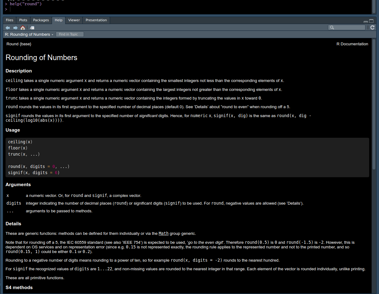
Figure 4.1: Documentation of the `round()` function. Preview of functions documentations looks like

4.2 Some Built-in Functions

There are many functions readily available in R to assist with your analysis tasks. For tasks that R’s built-in functions can’t handle, you can always install packages (covered in Chapter 7) or develop your custom functions, a concept we will cover in Section 4.3.

For examples, to know the total number of observations we have in tomato_weight we can use length().

length(tomato_weight)

[1] 10

To find the average of tomato_weight, we use mean().

mean(x = tomato_weight)

[1] 45.815

To check the median of the data use (you guessed it right) median(). We also have sd(), var(), and cor() for estimating the standard deviation, variance and correlation respectively.

median(tomato_weight)

[1] 42.545

sd(tomato_weight)

[1] 22.70789

var(tomato_weight)

[1] 515.6485

cor(tomato_weight, 1:10)

[1] -0.1669699

We’ve seen round() in action before. However round() is having two siblings . The ceiling() and floor() function to round up and down respectively.

floor(3.544)

[1] 3

ceiling(3.544)

[1] 4

To create a sequence of number, we can use colon (:).

20:30

 [1] 20 21 22 23 24 25 26 27 28 29 30

30:20

 [1] 30 29 28 27 26 25 24 23 22 21 20

This gives a sequence of numbers increased or decreased by 1. To get more control over the sequence you want to create use the seq() function. Important arguments of seq() to remember are from, to, and by.

seq(from = 1, to = 100, by = 1)

  [1]   1   2   3   4   5   6   7   8   9  10  11  12  13  14  15  16  17  18
 [19]  19  20  21  22  23  24  25  26  27  28  29  30  31  32  33  34  35  36
 [37]  37  38  39  40  41  42  43  44  45  46  47  48  49  50  51  52  53  54
 [55]  55  56  57  58  59  60  61  62  63  64  65  66  67  68  69  70  71  72
 [73]  73  74  75  76  77  78  79  80  81  82  83  84  85  86  87  88  89  90
 [91]  91  92  93  94  95  96  97  98  99 100

With positional argument, it could be written as shown below

seq(1, 100, 1)

R also comes with built-in constants such as pi , letters, LETTERS, month.abb and month.name

pi

[1] 3.141593

letters

 [1] "a" "b" "c" "d" "e" "f" "g" "h" "i" "j" "k" "l" "m" "n" "o" "p" "q" "r" "s"
[20] "t" "u" "v" "w" "x" "y" "z"

month.abb

 [1] "Jan" "Feb" "Mar" "Apr" "May" "Jun" "Jul" "Aug" "Sep" "Oct" "Nov" "Dec"

4.2.1 Simulating Numbers

Aside from generating sequence of numbers, we can simulate numbers using R to meet certain distributions. An important part of research is data simulation and R provides a robust set of functions for generating random numbers from different distributions. For example, the runif() function generates random numbers from a uniform distribution, rnorm() for the normal distribution, rpois() for the Poisson distribution, and rbinom() for the binomial distribution. These functions belong to a family that also includes functions for calculating density (d), distribution functions (p), quantiles (q), and random deviates (r) for various statistical distributions. A comprehensive list of these functions can be found in Table 4.1.

For example, to simulate the height of 100 Tectona grandis in a plantation with mean diameter of 35 cm and a standard deviation of 2.3 cm we use rnorm(). rnorm() generates random numbers following the normal distribution.

teak_diameter <- rnorm(100, mean = 35, sd = 2.3)
teak_diameter

  [1] 33.55793 29.83694 33.40181 39.62091 32.67943 34.52777 34.74032 36.04776
  [9] 35.30509 34.29091 32.99311 33.64304 31.25549 38.77401 31.53192 34.93754
 [17] 32.55688 38.68862 35.69456 33.69591 32.71016 33.54308 33.75140 34.89965
 [25] 33.06363 33.53775 35.30344 32.36311 35.38665 33.87271 33.87264 36.67399
 [33] 33.91518 34.73610 40.74431 35.10364 33.99462 35.36381 34.32652 38.77067
 [41] 38.97418 33.63464 34.94445 36.51109 35.20498 35.71871 34.30049 33.48404
 [49] 32.59673 39.80583 35.07444 34.05283 34.91802 33.57329 38.32692 35.96444
 [57] 33.79829 34.49797 36.29705 30.35382 36.48489 37.68427 34.62237 37.90798
 [65] 36.47568 32.89580 33.99327 35.84308 30.90215 33.21831 36.08523 33.82663
 [73] 32.30792 33.87001 36.23541 37.81431 37.95922 33.23668 33.79195 35.31234
 [81] 33.54759 35.54844 35.69272 33.59550 36.68904 37.18523 33.17504 36.25569
 [89] 35.49645 32.27447 37.26336 35.06208 35.47546 37.20467 34.15940 37.49995
 [97] 31.39632 38.90451 34.21432 34.59158

The numbers generated above will be different from that which you will produce. This is because they are random numbers. The beauty of R is its reproducibility, and what use is reproducibility if others can’t get the same result as us if they follow exactly the same steps as us. That’s why there’s the set.seed() function which captures or get a snapshot of specific numbers randomly generated. Given that the seed number is the same, whatever pseudorandom numbers are produce can be replicated by another person.

set.seed(123)
tree_diameter <- rnorm(100, mean = 25, sd = 12.3)
tree_diameter

  [1] 18.106150 22.168817 44.172112 25.867253 26.590239 46.095299 30.669269
  [8]  9.439747 16.551710 19.518358 40.056206 29.425710 29.929489 26.361397
 [15] 18.163154 46.979032 31.123561  0.810609 33.626678 19.184666 11.865768
 [22] 22.318909 12.380145 16.034638 17.312017  4.253672 35.304781 26.886489
 [29] 11.000916 40.421924 30.245510 21.370621 36.010046 35.801042 35.105447
 [36] 33.470275 31.813187 24.238486 21.236659 20.320207 16.455104 22.442617
 [43]  9.435625 51.678158 39.857933 11.185764 20.044517 19.260139 34.593571
 [50] 23.974560 28.115818 24.648875 24.472693 41.833808 22.223017 43.652588
 [57]  5.950341 32.190749 26.523407 27.656081 29.669566 18.821422 20.901549
 [64] 12.471523 11.816968 28.733402 30.512980 25.651952 36.343890 50.216042
 [71] 18.960317 -3.402777 37.370584 16.276831 16.537494 37.614528 21.497292
 [78]  9.985172 27.230033 23.291636 25.070899 29.738949 20.440882 32.925832
 [85] 22.288015 29.080918 38.491120 30.352732 20.991041 39.130334 37.220097
 [92] 31.745283 27.936400 17.276755 41.736025 17.616807 51.904196 43.851111
 [99] 22.100886 12.375023

With the seed set already, you should have exactly the same result as what is produced here.

We can understand the data which we just produced if it is visualized. With the plot() function, we can produce a graph. Not to worry we will cover more on visualizations Chapter 12.

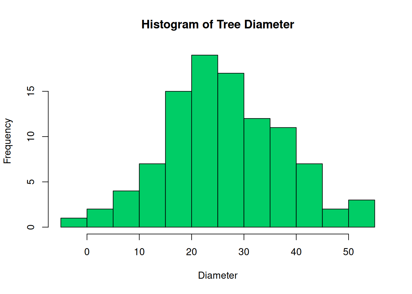
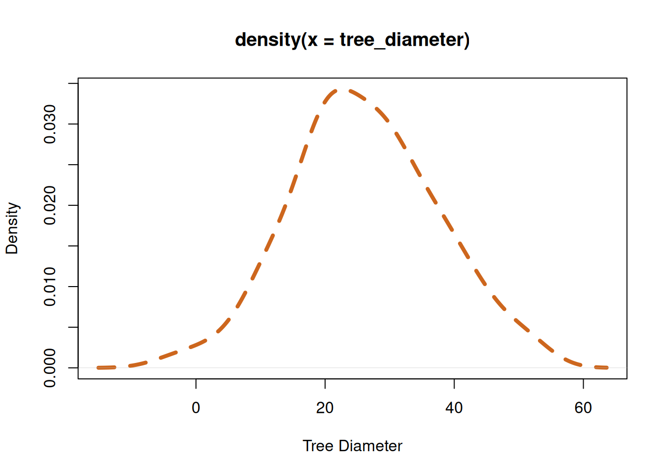
In forestry, the distribution of trees diameter in a plantation is usually a bell-shaped curve. Figure 4.2 (b) shows the distribution of the diameter, while the distribution of the diameters represented as a histogram can be seen in Figure 4.2 (a).

While rnorm() generates numbers that follow a normal distribution runif() generates numbers that follow a uniform distribution, Figure 4.3.

set.seed(123)
dt <- runif(100, min = 10, max = 20)
dt

  [1] 12.87578 17.88305 14.08977 18.83017 19.40467 10.45556 15.28105 18.92419
  [9] 15.51435 14.56615 19.56833 14.53334 16.77571 15.72633 11.02925 18.99825
 [17] 12.46088 10.42060 13.27921 19.54504 18.89539 16.92803 16.40507 19.94270
 [25] 16.55706 17.08530 15.44066 15.94142 12.89160 11.47114 19.63024 19.02299
 [33] 16.90705 17.95467 10.24614 14.77796 17.58460 12.16408 13.18181 12.31626
 [41] 11.42800 14.14546 14.13724 13.68845 11.52445 11.38806 12.33034 14.65962
 [49] 12.65973 18.57828 10.45831 14.42200 17.98925 11.21899 15.60948 12.06531
 [57] 11.27532 17.53308 18.95045 13.74463 16.65115 10.94841 13.83970 12.74384
 [65] 18.14640 14.48516 18.10064 18.12390 17.94342 14.39832 17.54475 16.29221
 [73] 17.10182 10.00625 14.75317 12.20119 13.79817 16.12771 13.51798 11.11135
 [81] 12.43619 16.68056 14.17647 17.88196 11.02865 14.34893 19.84957 18.93051
 [89] 18.86469 11.75053 11.30696 16.53102 13.43516 16.56758 13.20373 11.87691
 [97] 17.82294 10.93595 14.66779 15.11505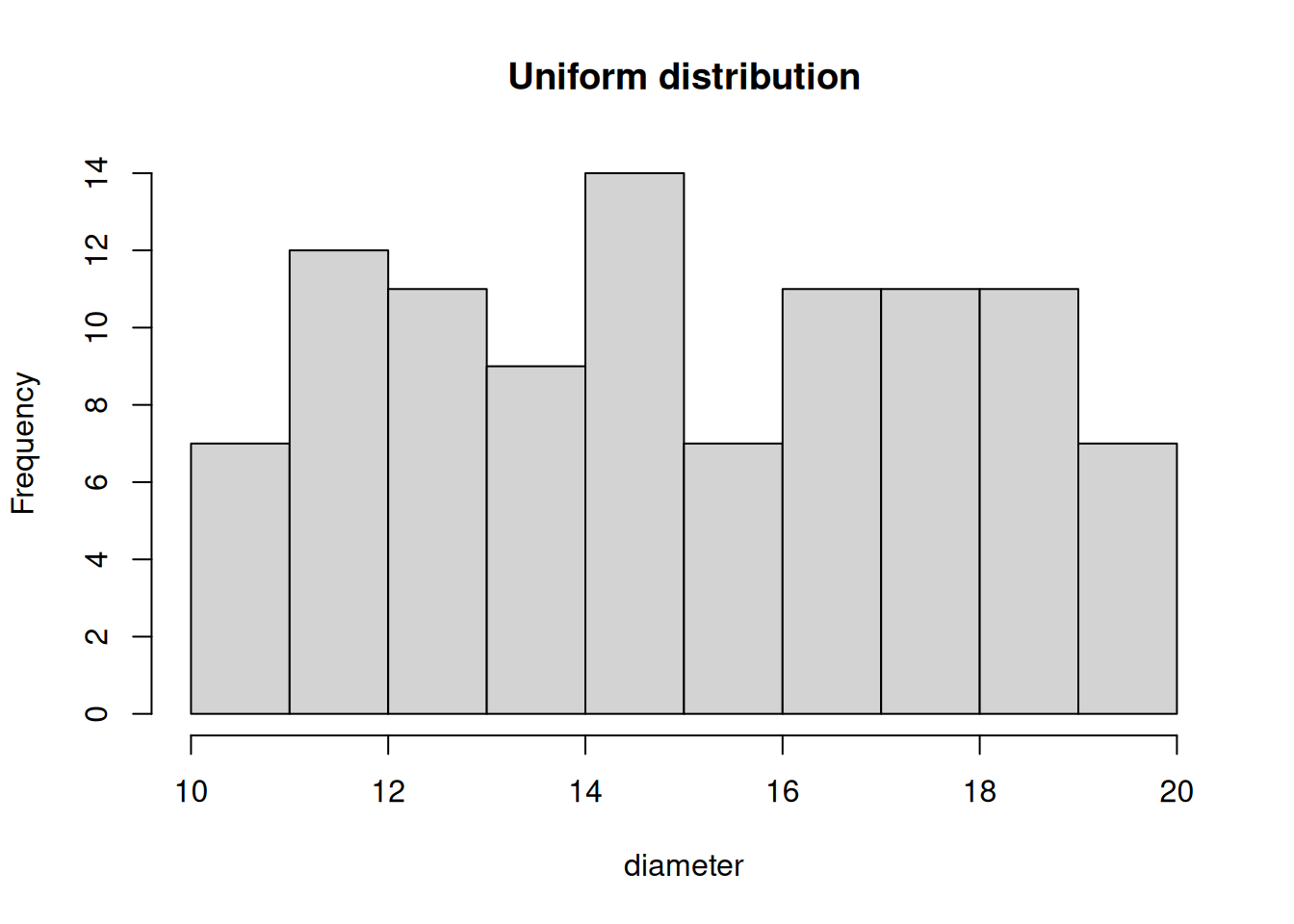

Figure 4.3: Uniformly distributed randomly generated numbers. The higher the number of observations the more uniform the distribution.

Other functions for generating random numbers according to distribution are:

Table 4.1: Functions for generating random numbers of data in R

Function	Distribution	Description
runif	Uniform distribution	Generates random numbers from a uniform distribution
rnorm	Normal distribution	Generates random numbers from a normal distribution
rpois	Poisson distribution	Generates random numbers from a poisson distribution
rbinom	Binomial distribution	Generates random numbers from a binomial distribution
dunif	Uniform distribution	Computes the density of a uniform distribution
dnorm	Normal distribution	Computes the density of a normal distribution
dpois	Poisson distribution	Computes the density of a poisson distribution
dbinom	Binomial distribution	Computes the density of a binomial distribution
punif	Uniform distribution	Computes the cumulative distribution function (CDF) of a uniform distribution
pnorm	Normal distribution	Computes the cumulative distribution function (CDF) of a normal distribution
ppois	Poisson distribution	Computes the cumulative distribution function (CDF) of a poisson distribution
pbinom	Binomial distribution	Computes the cumulative distribution function (CDF) of a binomial distribution
qunif	Uniform distribution	Computes the quantiles of a uniform distribution
qnorm	Normal distribution	Computes the quantiles of a normal distribution
qpois	Poisson distribution	Computes the quantiles of a poisson distribution
qbinom	Binomial distribution	Computes the quantiles of a binomial distribution

4.2.2 Sampling with sample()

Another important function for randomization is using sample(). sample() is used for selecting values at random from a set of data. Let’s take the example below:

new_dt <- seq(1, 20, 2)
new_dt

 [1]  1  3  5  7  9 11 13 15 17 19

We can randomly select five values from new_dt using sample()

set.seed(10)
sample(new_dt, 5)

[1] 17 13 15 11  5

The sample() function is used for simulating die roll, coin toss, and even draws from a stack of card. For example, we can simulate the number we get from a die with the following:

die <- 1:6

sample(die, 1)

[1] 2

If you continue to run the code above, you will continue to get different values. A good challenge for you would be to simulate two die.

4.2.2.1 Weighted Samples and Sampling with Replacement

More than selecting values at random, with sample(), we can also select with replacement by setting the value of the argument replace to TRUE.

sample(new_dt, 20, replace = TRUE)

 [1] 13 19  3 15 15 13 11 13 11  3  9 17  3 19  9 19  1 13 19  3

The probabilities of the values we want to randomly select can also be determined by the prob argument. This is perfect for weighted probability. Example is a die of unequal prob.

die <- 1:6
die_prob <- c(0.23, 0.23, 0.23, 0.21, 0.07, 0.03)

set.seed(123)
die_selected <- sample(x = die, size = 100, replace = TRUE, prob = die_prob)
die_selected

  [1] 1 4 1 4 5 2 3 4 3 1 5 1 3 3 2 4 1 2 1 5 4 4 3 6 3 4 3 3 1 2 5 5 4 4 2 3 4
 [38] 2 1 1 2 1 1 1 2 2 1 3 1 4 2 1 4 2 3 2 2 4 4 1 3 2 1 1 4 1 4 4 4 1 4 3 4 2
 [75] 3 2 1 3 1 2 1 3 1 4 2 1 6 4 4 2 2 3 1 3 1 2 4 2 3 3

To get the number of occurrence of each die face we can use the table() function. and notice that values with lower probability of occurring such as 5 and 6 were sampled less.

table(die_selected)

die_selected
 1  2  3  4  5  6 
27 22 20 24  5  2

4.2.3 Character Functions

We’ve been working with numbers for a while, now lets see some functions that we can use for character data types. To begin, let’s create a vector of character data type.

tree_1 <- "Adansonia digitata"
tree_1

[1] "Adansonia digitata"

4.2.3.1 Counting Characters

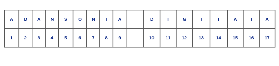
Counting character is done using nchar(). Whenever, we count characters, we usually neglect the space and as such when we count the tree_1 object we should expect 17 characters as what we have in Figure 4.4.

Figure 4.4: Number of characters in the object if counted without the space

Using nchar() we get a different result.

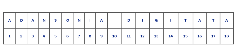
nchar(tree_1)

[1] 18

This might come as a surprise. This is because spaces are also counted as characters, not only in R, but also in word processors like Microsoft Word or LibreOffice Writer and other programming languages. Given that, Figure 4.5 shows the actual number of characters with spaces included.

Figure 4.5: Number of characters in the object with the spaces included

Characters can also be changed to lower cases by using tolower(), and changed to upper cases by using toupper(). Unfortunately, Base R does not provide a function to changed strings to title or sentence cases, but there are open source packages available to do this . You can explore stringr by Hadley Wickham and stringi by Marek Gagolewski which contains functions for such operation and other complex string manipulation operations in R.

tolower(tree_1)

[1] "adansonia digitata"

toupper(tree_1)

[1] "ADANSONIA DIGITATA"

4.2.3.2 Trimming Characters

There are some data where part of the variable are filled by respondents. This can include records of names, for example, clinic require records of physicians and the name of their patients. A particular physician could attend to multiple patient in a day and at different times in a day. Below is an example of physicians name in a clinic working different times. e could have the names of five clinic physicians repeated multiple times, according to the number of times they have shifts, or attend to patients.

physician <- c("Clara Reeves", "Motolani Eniola", "Praaval Duval", " Praaval Duval ", "Sunmisola Aderibigbe ", " Sunmisola Aderibigbe"," Clara Reeves", "Clara Reeves ", " Motolani Eniola ", "Praaval Duval ")

physician

 [1] "Clara Reeves"          "Motolani Eniola"       "Praaval Duval"        
 [4] " Praaval Duval "       "Sunmisola Aderibigbe " " Sunmisola Aderibigbe"
 [7] " Clara Reeves"         "Clara Reeves "         " Motolani Eniola "    
[10] "Praaval Duval "

The example above is a classic example of having white spaces. We can check the data to see the number of distinct physicians we have.

length(unique(physician))

[1] 10

This returns 10 but we can see clearly that some names just has extra white spaces. With the trimws() function we could remove excess white spaces in the data. Before using the function lets count the number of characters we have for each observation. We will do the same after trimming to see the difference.

nchar(physician)

 [1] 12 15 13 15 21 21 13 13 17 14

physician_trimmed <- trimws(physician)
physician_trimmed

 [1] "Clara Reeves"         "Motolani Eniola"      "Praaval Duval"       
 [4] "Praaval Duval"        "Sunmisola Aderibigbe" "Sunmisola Aderibigbe"
 [7] "Clara Reeves"         "Clara Reeves"         "Motolani Eniola"     
[10] "Praaval Duval"

nchar(physician_trimmed)

 [1] 12 15 13 13 20 20 12 12 15 13

Now we can tell the number of characters reduced for most of the observations. We can now confirm the number of physicians we have using length() and unique().

length(unique(physician_trimmed))

[1] 4

The four physicians are:

unique(physician_trimmed)

[1] "Clara Reeves"         "Motolani Eniola"      "Praaval Duval"       
[4] "Sunmisola Aderibigbe"

The technique taught here is very useful in the data cleaning process.

4.2.3.3 Extracting and Replacing Part(s) of a Chaaracter

To extract certain aspect of your text, use substring(), or substr(). substr() takes the argument x which is your data, start which is the index position for the first value of the text to be extracted or replaced, and stop which is the index position for the last value of the text to be extracted or replaced. For example, we can extract Adansonia from the text with the following code.

substr(tree_1, start = 1, stop = 9)

[1] "Adansonia"

To replace a certain part of the text we can also use substr().

substr(tree_1, start = 11, nchar(tree_1)) <- "gregorii"
tree_1

[1] "Adansonia gregorii"

There are times, we would like to split text data, using strsplit(). For example we can split the tree_1 to genus and species with the spaces between them.

strsplit(tree_1, split = " ")

[[1]]
[1] "Adansonia" "gregorii"

Notice the output, both words now have their inverted comma.

There are still more functions for string manipulation in R, not all will be covered, as this will be a large book volume.

4.3 Custom Functions

The functions that are preloaded in R are a lot, but that does not mean they will meet all our statistical or operational needs. For some tasks you want to do, you would need to write your own function.

4.3.1 Creating Custom Functions

For example we can estimate the z-score of the tomato_weight data. The z-score tells you how many standard deviations an element is from the mean of the vector. It transforms our data into a common scale. The formula for z-score is given as:

\(Z = \frac{x - \mu}{\sigma}\)

Where:

\(x\) is the value in the vector,
\(\mu\) is the mean of the vector,
\(\sigma\) is the standard deviation of the vector.

Without a custom function we will do the following:

average_tomato <- mean(tomato_weight)
sd_tomato <- sd(tomato_weight)
z_tomato <- (tomato_weight - average_tomato) / sd_tomato

average_tree_diameter <- mean(tree_diameter)
sd_tree_diameter <- sd(tree_diameter)
z_tree_diameter <- (tree_diameter - average_tree_diameter) / sd_tree_diameter

average_dt <-mean(dt)
sd_tomato <- sd(dt)
z_dt <- (dt - average_dt) / sd_tomato

We got the following results

z_tomato

 [1] -0.09402017  1.07517674 -0.72683973  1.64105924 -0.81007070  0.33842856
 [7] -0.65461816 -1.55474564 -0.19398540  0.97961526

z_tree_diameter

  [1] -0.71304802 -0.35120270  1.60854170 -0.02179795  0.04259548  1.77983218
  [7]  0.40589817 -1.48492941 -0.85149566 -0.58726835  1.24195461  0.29513939
 [13]  0.34000892  0.02221347 -0.70797086  1.85854263  0.44636008 -2.25349176
 [19]  0.66930255 -0.61698896 -1.26885349 -0.33783464 -1.22304003 -0.89754917
 [25] -0.78377819 -1.94683206  0.81876439  0.06898128 -1.34588242  1.27452758
 [31]  0.36815564 -0.42229479  0.88157948  0.86296437  0.80101058  0.65537241
 [37]  0.50778230 -0.16686565 -0.43422620 -0.51585092 -0.86009994 -0.32681639
 [43] -1.48529653  2.27707482  1.22429519 -1.32941869 -0.54040552 -0.61026684
 [49]  0.75541982 -0.19037243  0.17847258 -0.13031397 -0.14600575  1.40027842
 [55] -0.34637532  1.56226982 -1.79571669  0.54141021  0.03664303  0.13752572
 [61]  0.31685861 -0.64934164 -0.46407310 -1.21490140 -1.27319995  0.23347834
 [67]  0.39197814 -0.04097396  0.91131364  2.14685001 -0.63697081 -2.62876100
 [73]  1.00275711 -0.87597805 -0.85276181  1.02448422 -0.41101270 -1.43635058
 [79]  0.09957931 -0.25119772 -0.09272595  0.32303830 -0.50510289  0.60688103
 [85] -0.34058618  0.26443017  1.10255872  0.37770550 -0.45610238  1.15949090
 [91]  0.98935390  0.50173432  0.16249260 -0.78691881  1.39156928 -0.75663177
 [97]  2.29720706  1.57995139 -0.35725306 -1.22349625

z_dt

  [1] -0.74029816  1.01667000 -0.31432828  1.34899927  1.55058114 -1.58950882
  [7]  0.10367363  1.38198803  0.18553298 -0.14717528  1.60800687 -0.15868628
 [13]  0.62812145  0.25991452 -1.38821361  1.40797416 -0.88587877 -1.60177908
 [19] -0.59874073  1.59983236  1.37188355  0.68157065  0.49807079  1.73936495
 [25]  0.55140145  0.73675424  0.15967644  0.33538461 -0.73474643 -1.23316204
 [31]  1.62972964  1.41665527  0.67420868  1.04180123 -1.66299360 -0.07285392
 [37]  0.91194687 -0.99002015 -0.63291572 -0.93662330 -1.24829781 -0.29478615
 [43] -0.29767044 -0.45514279 -1.21445611 -1.26231194 -0.93168176 -0.11437574
 [49] -0.81610602  1.26061293 -1.58854506 -0.19775388  1.05393276 -1.32163504
 [55]  0.21891237 -1.02467527 -1.30187194  0.89387052  1.39120332 -0.43543256
 [61]  0.58441742 -1.41657907 -0.40207459 -0.78659323  1.10907471 -0.17559117
 [67]  1.09301940  1.10117798  1.03785346 -0.20606415  0.89796636  0.45847125
 [73]  0.74255060 -1.74716662 -0.08155371 -0.97699906 -0.41664711  0.40075054
 [79] -0.51495972 -1.35940351 -0.89453948  0.59473476 -0.28390722  1.01628648
 [85] -1.38842427 -0.22339407  1.70668793  1.38420585  1.36111055 -1.13512882
 [91] -1.29076986  0.54226490 -0.54401788  0.55509389 -0.62522354 -1.09078258
 [97]  0.99557901 -1.42094993 -0.11151046  0.04542695

If we look closely, we can spot an error while computing z_dt. The following steps can be done easily with a custom function. To create a custom function we need to solidify our understanding of functions. In R, every functions have three basic parts; a name, a body, and set of arguments. To create functions in R we call function() function followed by {}.

new_function <- function() {}

The name of the arguments is passed into the parenthesis of function() and the body, or expresions are passed into the curly brackets.

z_score <- function(x) {
  average_x <- mean(x, na.rm = TRUE)
  sd_x <- sd(x, na.rm = TRUE)
  z_value = (x - average_x)/sd_x
  return(z_value)
}

Next is using the custom function. We should note that, custom functions are called in a similar way that R’s built-in functions are called, the object name followed by parenthesis.

z_tomato_2 <- z_score(tomato_weight)
z_tomato_2

 [1] -0.09402017  1.07517674 -0.72683973  1.64105924 -0.81007070  0.33842856
 [7] -0.65461816 -1.55474564 -0.19398540  0.97961526

z_tree_diameter_2 <- z_score(tree_diameter)
z_tree_diameter_2

  [1] -0.71304802 -0.35120270  1.60854170 -0.02179795  0.04259548  1.77983218
  [7]  0.40589817 -1.48492941 -0.85149566 -0.58726835  1.24195461  0.29513939
 [13]  0.34000892  0.02221347 -0.70797086  1.85854263  0.44636008 -2.25349176
 [19]  0.66930255 -0.61698896 -1.26885349 -0.33783464 -1.22304003 -0.89754917
 [25] -0.78377819 -1.94683206  0.81876439  0.06898128 -1.34588242  1.27452758
 [31]  0.36815564 -0.42229479  0.88157948  0.86296437  0.80101058  0.65537241
 [37]  0.50778230 -0.16686565 -0.43422620 -0.51585092 -0.86009994 -0.32681639
 [43] -1.48529653  2.27707482  1.22429519 -1.32941869 -0.54040552 -0.61026684
 [49]  0.75541982 -0.19037243  0.17847258 -0.13031397 -0.14600575  1.40027842
 [55] -0.34637532  1.56226982 -1.79571669  0.54141021  0.03664303  0.13752572
 [61]  0.31685861 -0.64934164 -0.46407310 -1.21490140 -1.27319995  0.23347834
 [67]  0.39197814 -0.04097396  0.91131364  2.14685001 -0.63697081 -2.62876100
 [73]  1.00275711 -0.87597805 -0.85276181  1.02448422 -0.41101270 -1.43635058
 [79]  0.09957931 -0.25119772 -0.09272595  0.32303830 -0.50510289  0.60688103
 [85] -0.34058618  0.26443017  1.10255872  0.37770550 -0.45610238  1.15949090
 [91]  0.98935390  0.50173432  0.16249260 -0.78691881  1.39156928 -0.75663177
 [97]  2.29720706  1.57995139 -0.35725306 -1.22349625

z_dt_2 <- z_score(dt)
z_dt_2

  [1] -0.74029816  1.01667000 -0.31432828  1.34899927  1.55058114 -1.58950882
  [7]  0.10367363  1.38198803  0.18553298 -0.14717528  1.60800687 -0.15868628
 [13]  0.62812145  0.25991452 -1.38821361  1.40797416 -0.88587877 -1.60177908
 [19] -0.59874073  1.59983236  1.37188355  0.68157065  0.49807079  1.73936495
 [25]  0.55140145  0.73675424  0.15967644  0.33538461 -0.73474643 -1.23316204
 [31]  1.62972964  1.41665527  0.67420868  1.04180123 -1.66299360 -0.07285392
 [37]  0.91194687 -0.99002015 -0.63291572 -0.93662330 -1.24829781 -0.29478615
 [43] -0.29767044 -0.45514279 -1.21445611 -1.26231194 -0.93168176 -0.11437574
 [49] -0.81610602  1.26061293 -1.58854506 -0.19775388  1.05393276 -1.32163504
 [55]  0.21891237 -1.02467527 -1.30187194  0.89387052  1.39120332 -0.43543256
 [61]  0.58441742 -1.41657907 -0.40207459 -0.78659323  1.10907471 -0.17559117
 [67]  1.09301940  1.10117798  1.03785346 -0.20606415  0.89796636  0.45847125
 [73]  0.74255060 -1.74716662 -0.08155371 -0.97699906 -0.41664711  0.40075054
 [79] -0.51495972 -1.35940351 -0.89453948  0.59473476 -0.28390722  1.01628648
 [85] -1.38842427 -0.22339407  1.70668793  1.38420585  1.36111055 -1.13512882
 [91] -1.29076986  0.54226490 -0.54401788  0.55509389 -0.62522354 -1.09078258
 [97]  0.99557901 -1.42094993 -0.11151046  0.04542695

Using a custom function does not only make our code more readable, it prevents errors from copying and pasting, and if we need to make a change in out formula, we need to do it in only a place–the function definition.

4.3.2 When to Write a Custom Functiom

When do you need to write a function?

When you find yourself copying, pasting and adapting blocks of code. Copying, pasting and adapting codes to new data or objects should not be more than three times.
When the code is clunky and not readable, writing custom functions improves the readability of your code
For individuals that regular submit report to different people, stakeholders, and groups, parametizing different inputs in your report ensure you produce multiple focused report at once.
Avoiding code duplication

Getting Help

Use the help() function and ? to get help. Also, use args() to see the arguments of functions. Just to let you know, there are more than 2300 functions loaded when an R session starts and that’s a lot. You will remember some and forget some, but as keep using R they become a part of you.

You are not expected to remember these functions, use help(), ? and args() and check online for resources when you need help.

4.4 Summary

Functions are little codes that performs specific functions. Armed with them we can fly on eagles wing. Functions such as mean(), length(), plot() and so on, makes it easier to perform tasks. However, this does not imply that there are functions for all tasks we want to accomplish. In such case, we need to develop our own functions called, custom functions. There are also functions in other packages which extends the capabilities of R.

Exercise

Using seq(), create a sequence of odd numbers between 1 and 100.
Read the documentation of mean(), median(), sd(), and var(). What does the is.na() argument does?
What is the difference between substring() and substr()?
What is the difference between paste() and paste0()?