library(pacman)
p_load(readr, data.table)10 Getting External Data into RStudio
When working in the data field, you are more likely to get the data from external sources than record it manually yourself, and being honest, recording your data in R is a big task, especially when it is large. While it’s difficult to record data in R, it is possible using edit() which opens an empty box for you to input data. Good thing is that lab equipment have features that makes them record data as they are measured. These recorded data can later be exported as spreadsheet file or plain-text files.
10.1 Important Concepts
Before we go into data importation, it is important we understand some concepts that will make this process easy and less error prone.
10.1.1 Data Sources
When we want to import data into R, we need to know where to get it from. A data source is the place where the data we want to use originates from. This can be a physical or digital place A data source could be any of a live measurements from physical devices, a database, a flat file or plain-text file, scraped web data, or any of the innumerable static and streaming data services which abound across the internet. An example of a data source is data.gov, and wikipedia and these are web data. Another example that is actually close to you is your mobile phone. It’s a mobile database holding contact information, music data, games, and so on.
10.1.2 Data Format
Data formats represent the form, structure and organization of data. It defines how information is stored, accessed, and interpreted. It’s a standardized way to represent data, whether in files or databases, and is crucial for efficient data management and processing. This brings us to another aspect that is important to knowing how to handle data, and that’s file extension. If you’ve taken a closer look at the music/audio file on any of your device, you usually see a dot which separates the name of the file and a text which is usually fairly consistent depending on your file organization. This text is regarded to as the file extension. This is also true for your video, and picture files. For example, you could see the following extensions:
| Audio | Pictures | Video |
|---|---|---|
| .mp3 | .png | .mp4 |
| .aac | .jpeg | .mov |
| .flac | .gif | .avi |
| .wav | .webp | .web, |
| .ogg | .tiff | .mov |
For data set, there are some common file format such as:
- flat file :
.csv,.tsv,.txt,.rtf - some web data format excluding those above:
.html,.json,xml - spreadsheet:
.xlsx,.xls,.xlsm,.ods,.gsheet - others:
.shp,.hdsf,.sav, and many more.
10.2 Importing Data {sec-import-section}
Data is imported into R based on the file format you are dealing with. We will import some of the file types you would come across when working with data in R.
10.3 Flat file data
Flat files are one of the most common forms in which data are stored. They are basically text files with a consistent structure. To import text files, we can use either of base R utils, data.table or readr. There are still other packages that we can use to import flat files, but, the ones provided here should be sufficient for any flat file. Firstly let’s import pacman and use it’s p_load() function to import the packages we need. If you do not have pacman installed, you can use install.packages( "< package name >" ) to do so.
pacman makes data importation and management very easy. It makes download easy without the need for quotation marks as required when using install.packages(). It also has the p_load() function which is used to download, install, and load packages at the same time, performing the function of install.packages, and library at once.
Without pacman, the steps would be:
install.packages(c("data.table", "readr")) # this can be further broken down
library(data.table)
library(readr)
This is what makes pacman shines to me. You could also run the below, if you do not want to load pacman itself but just make use of its function.
pacman::p_load(readr, data.table)Now that we are done with installing and loading our packages, let’s take a closer look at the different flat files. There are two things we should consider when dealing with flat files:
- The extension of the file.
- The structure of file when opened.
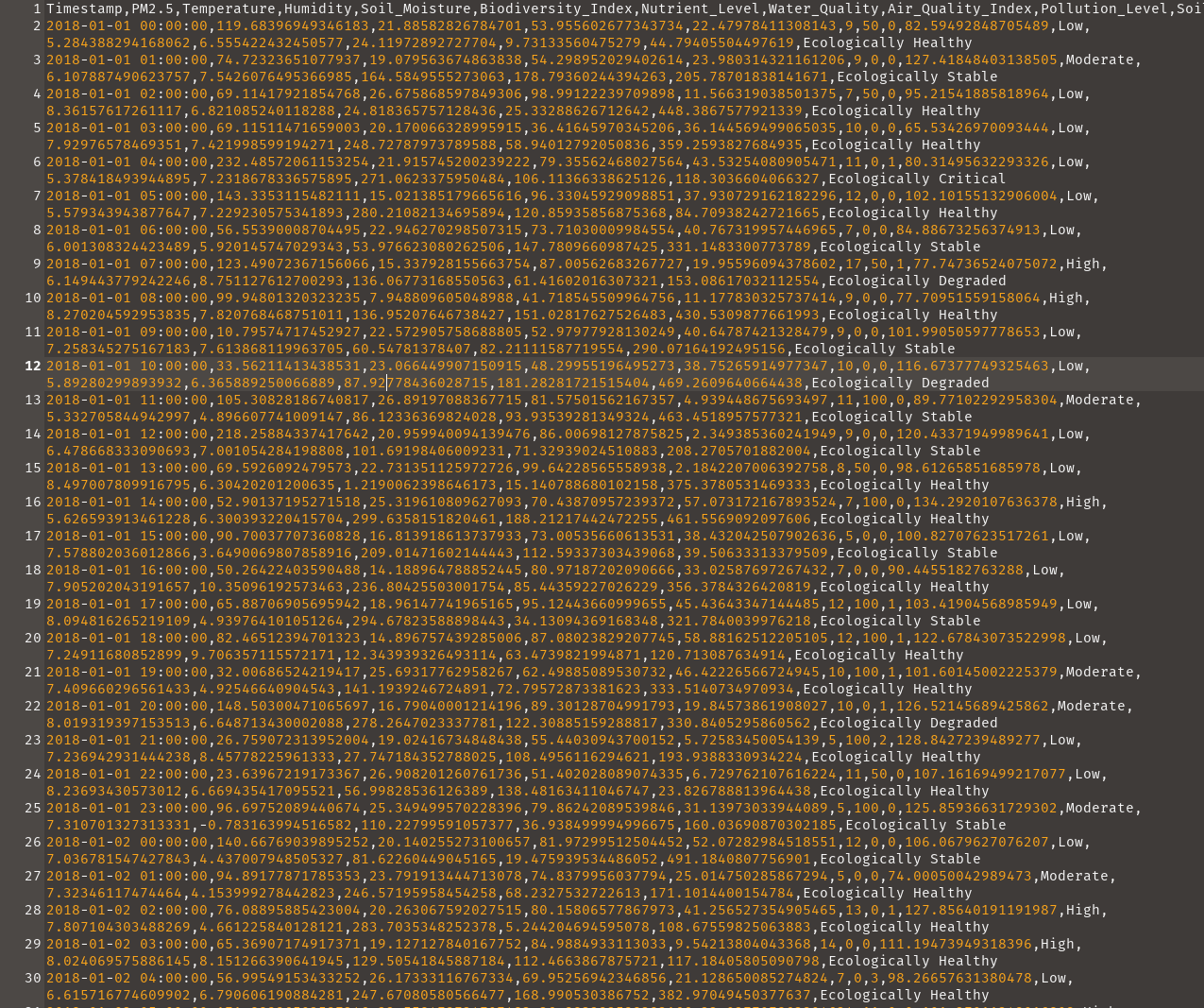
To some degree, the extension of your file could give you a hint on how to read it into R. .csv, would need a csv file reading function, .txt, would need its own also. Notwithstanding, the internal structure is what makes reading a file easier. In flat files data, the data presented in a way that mimics standard spreadsheet table, with the difference being in how their recorded are separated. While a spreadsheet is having its rows and column clearly defined, flat files have its own separated using a consistent sign or symbol in the document. These signs and symbols are regarded to as delimiters. For example, Figure 10.1 have it’s columns separated by commas, so the delimiter is a comma, thus the name comma separated values.
If it is separated by semi-colon, the delimiter is a semi colon, but the name remains the same. The interesting thing is that comma separated files can still have their name saved in .txt format, that’s why checking the file internal structure is important. Although almost anything can be used as a delimiter. Some common ones includes:
- comma -
, - tab -
\t - semicolon -
; - pipe -
|, - whitespace
To read a csv into R, you can run any of the following. They all have a first common argument which is the file path:
# Base R implementation

my_data <- read.csv(file = "data/ecological_health_dataset.csv")

head(my_data)
Timestamp PM2.5 Temperature Humidity Soil_Moisture
1 2018-01-01 00:00:00 119.68397 21.88583 53.95560 22.47978
2 2018-01-01 01:00:00 74.72324 19.07956 54.29895 23.98031
3 2018-01-01 02:00:00 69.11418 26.67587 98.99122 11.56632
4 2018-01-01 03:00:00 69.11511 20.17007 36.41646 36.14457
5 2018-01-01 04:00:00 232.48572 21.91575 79.35562 43.53254
6 2018-01-01 05:00:00 143.33531 15.02139 96.33046 37.93073
Biodiversity_Index Nutrient_Level Water_Quality Air_Quality_Index
1 9 50 0 82.59493
2 9 0 0 127.41848
3 7 50 0 95.21542
4 10 0 0 65.53427
5 11 0 1 80.31496
6 12 0 0 102.10155
Pollution_Level Soil_pH Dissolved_Oxygen Chemical_Oxygen_Demand
1 Low 5.284388 6.555422 24.11973
2 Moderate 6.107887 7.542608 164.58496
3 Low 8.361576 6.821085 24.81837
4 Low 7.929766 7.421999 248.72788
5 Low 5.378418 7.231868 271.06234
6 Low 5.579344 7.229231 280.21082
Biochemical_Oxygen_Demand Total_Dissolved_Solids Ecological_Health_Label
1 9.731336 44.79406 Ecologically Healthy
2 178.793602 205.78702 Ecologically Stable
3 25.332886 448.38676 Ecologically Healthy
4 58.940128 359.25938 Ecologically Healthy
5 106.113663 118.30366 Ecologically Critical
6 120.859359 84.70938 Ecologically Healthy
head()returns the firsts 6 records of the dataset.
The readr implementation is also quite straight forward, instead of read.csv() it uses read_csv().
readr's read_csv. Produces a tibble instead of a data.frame.
read_csv("data/ecological_health_dataset.csv") |> head()Rows: 61345 Columns: 16
── Column specification ────────────────────────────────────────────────────────
Delimiter: ","
chr (2): Pollution_Level, Ecological_Health_Label
dbl (13): PM2.5, Temperature, Humidity, Soil_Moisture, Biodiversity_Index, ...
dttm (1): Timestamp
ℹ Use `spec()` to retrieve the full column specification for this data.
ℹ Specify the column types or set `show_col_types = FALSE` to quiet this message.# A tibble: 6 × 16
Timestamp PM2.5 Temperature Humidity Soil_Moisture
<dttm> <dbl> <dbl> <dbl> <dbl>
1 2018-01-01 00:00:00 120. 21.9 54.0 22.5
2 2018-01-01 01:00:00 74.7 19.1 54.3 24.0
3 2018-01-01 02:00:00 69.1 26.7 99.0 11.6
4 2018-01-01 03:00:00 69.1 20.2 36.4 36.1
5 2018-01-01 04:00:00 232. 21.9 79.4 43.5
6 2018-01-01 05:00:00 143. 15.0 96.3 37.9
# ℹ 11 more variables: Biodiversity_Index <dbl>, Nutrient_Level <dbl>,
# Water_Quality <dbl>, Air_Quality_Index <dbl>, Pollution_Level <chr>,
# Soil_pH <dbl>, Dissolved_Oxygen <dbl>, Chemical_Oxygen_Demand <dbl>,
# Biochemical_Oxygen_Demand <dbl>, Total_Dissolved_Solids <dbl>,
# Ecological_Health_Label <chr>This will be the first time we are seeing the operator |>. It is called the pipe operator and takes the result from its left hand side to the function/operation on the right hand side for evaluation. It is a nice way to chain operations without the need to break down your code. The above could be written as:
# Written as this
my_data <- read_csv("data/ecological_health_dataset.csv")
head(my_data)
# Or
head(read_csv("data/ecological_health_dataset.csv"))The pipe will be used alot moving forward so we get used to it.
The result of read_csv(), and read.csv() seems different, and that’s because one is a tibble–often regarded as the modern and clean version of data.frame–and the other is a data.frame. They show the same data with difference in presentation. The tibble is more detail and displays information about the dimension of the data, its column specification, then the data itself with each data type displayed under the column name. To learn more about tibble visit the Tibbles chapter in the R for Data Science 2nd Edition Book.
Next is data.table implementation of reading files. It is the easiest, and fastest of all three when it comes to data reading, and we will see that later on in time. It uses the function fread().
fread("data/ecological_health_dataset.csv") |>
head() Timestamp PM2.5 Temperature Humidity Soil_Moisture
<POSc> <num> <num> <num> <num>
1: 2018-01-01 00:00:00 119.68397 21.88583 53.95560 22.47978
2: 2018-01-01 01:00:00 74.72324 19.07956 54.29895 23.98031
3: 2018-01-01 02:00:00 69.11418 26.67587 98.99122 11.56632
4: 2018-01-01 03:00:00 69.11511 20.17007 36.41646 36.14457
5: 2018-01-01 04:00:00 232.48572 21.91575 79.35562 43.53254
6: 2018-01-01 05:00:00 143.33531 15.02139 96.33046 37.93073
Biodiversity_Index Nutrient_Level Water_Quality Air_Quality_Index
<int> <int> <int> <num>
1: 9 50 0 82.59493
2: 9 0 0 127.41848
3: 7 50 0 95.21542
4: 10 0 0 65.53427
5: 11 0 1 80.31496
6: 12 0 0 102.10155
Pollution_Level Soil_pH Dissolved_Oxygen Chemical_Oxygen_Demand
<char> <num> <num> <num>
1: Low 5.284388 6.555422 24.11973
2: Moderate 6.107887 7.542608 164.58496
3: Low 8.361576 6.821085 24.81837
4: Low 7.929766 7.421999 248.72788
5: Low 5.378418 7.231868 271.06234
6: Low 5.579344 7.229231 280.21082
Biochemical_Oxygen_Demand Total_Dissolved_Solids Ecological_Health_Label
<num> <num> <char>
1: 9.731336 44.79406 Ecologically Healthy
2: 178.793602 205.78702 Ecologically Stable
3: 25.332886 448.38676 Ecologically Healthy
4: 58.940128 359.25938 Ecologically Healthy
5: 106.113663 118.30366 Ecologically Critical
6: 120.859359 84.70938 Ecologically HealthyOf the three implementations, only the tibbles limits the column display to only what the screen/document can contain at a point in time, while the others have no limits.
Sometimes we do have files that we want to import that are available online. These functions read online files without trouble, just ensure you know the file extension, so your data gets imported as expected. The import speed now depends on your internet speed and the file size.
read_csv("https://raw.githubusercontent.com/EU-Study-Assist/data-for-r4r/refs/heads/main/r4r-II/prep-notes/data/ecological_health_dataset.csv") |>
head()`curl` package not installed, falling back to using `url()`
Rows: 61345 Columns: 16
── Column specification ────────────────────────────────────────────────────────
Delimiter: ","
chr   (2): Pollution_Level, Ecological_Health_Label
dbl  (13): PM2.5, Temperature, Humidity, Soil_Moisture, Biodiversity_Index, ...
dttm  (1): Timestamp

ℹ Use `spec()` to retrieve the full column specification for this data.
ℹ Specify the column types or set `show_col_types = FALSE` to quiet this message.
# A tibble: 6 × 16
Timestamp PM2.5 Temperature Humidity Soil_Moisture
<dttm> <dbl> <dbl> <dbl> <dbl>
1 2018-01-01 00:00:00 120. 21.9 54.0 22.5
2 2018-01-01 01:00:00 74.7 19.1 54.3 24.0
3 2018-01-01 02:00:00 69.1 26.7 99.0 11.6
4 2018-01-01 03:00:00 69.1 20.2 36.4 36.1
5 2018-01-01 04:00:00 232. 21.9 79.4 43.5
6 2018-01-01 05:00:00 143. 15.0 96.3 37.9
# ℹ 11 more variables: Biodiversity_Index <dbl>, Nutrient_Level <dbl>,
# Water_Quality <dbl>, Air_Quality_Index <dbl>, Pollution_Level <chr>,
# Soil_pH <dbl>, Dissolved_Oxygen <dbl>, Chemical_Oxygen_Demand <dbl>,
# Biochemical_Oxygen_Demand <dbl>, Total_Dissolved_Solids <dbl>,
# Ecological_Health_Label <chr>In addition to read.csv or read_csv, we have other read functions that are named according to their file extensions. A list of some read_* functions are give below. There’s a super function that reads a lot of flat file, that’s the read.delim or read_delim, you only have to specify your delimiter in the right argument–sep for read.delim() and delim for read_delim.
| file extension | base R | readr | data.table |
|---|---|---|---|
| txt | read.table | read.table | fread |
| tsv | read.delim | read_tsv | fread |
| dat | read.table | read_table | fread |
| log | readLines | read_lines | fread |
| tab | read.delim | read_delim | fread |
| psv | read.table | read_delim | fread |
| fixed-width | read.fwf | read_fwf | fread |
The good thing about data.table fread is that it guesses delimiter for its user, making it easier to import files. This in addition to how fast the package is, make it a useful package to learn.
There are other useful arguments you should take note off when you are importing data. Reading the documentation by using help() would expose you to these arguments. This include arguments like, header/col_names, sep/delim, na, skip, etc.
10.4 SpreadSheet
Base R, readr, and data.table cannot import spreadsheet data. Instead, packages are used. When we hear spreadsheet, MS Excel is the first thing that comes to mind–well maybe that’s my mind–but, spreadsheet are also different, and we can tell this by their file extensions. We have ods, xlsx, xls, gsheet. Except from gsheet which is usually a link in its non-native format, the rest can be seen as you tradition file extension on your personal computer.